Unlocking the Potential of Machine Learning in Econometrics: Ensemble Models for Improved…

Unlocking the Potential of Machine Learning in Econometrics: Ensemble Models for Improved Predictions with Limited Dataset

Introduction

With more and more data available today, large datasets are often used to gain insights in many fields, including economics. Yet, in econometrics, we often have to work with smaller datasets. This can make it difficult to use traditional machine learning methods. In this tutorial, we’ll explore how we can optimize these techniques using Ensemble models, enhancing our ability to extract valuable information even from limited data

GDP Per Capita

Gross Domestic Product (GDP) per capita is a widely used economic indicator that measures the average economic output per person in a country. It is calculated by dividing the total GDP of a nation by its population. GDP per capita provides valuable insights into the standard of living and economic well-being of the population. Economists are particularly interested in GDP per capita as it serves as a key metric for comparing the economic performance and development levels of different countries over time

Data Collection and Exploration

To begin, we gather economic data using the World Bank API, focusing on GDP per capita as the dependent variable (Y) and selecting a set of independent variables (X). These indicators, such as exports of goods and services, gross fixed capital formation, and energy use per capita, play significant roles in influencing GDP per capita. We analyze their correlation with GDP per capita, providing economic background insights into their impact

import pandas as pd
import wbdata
from pycaret.regression import *
from sklearn.model_selection import train_test_split
import seaborn as sns
import matplotlib.pyplot as plt
from sklearn.preprocessing import MinMaxScaler
from scipy.signal import argrelextrema

country_code = "USA"

indicators = {
    "NY.GDP.PCAP.CD": "GDP per capita",
    "SL.UEM.TOTL.ZS": "Unemployment rate",
    "EG.USE.PCAP.KG.OE": "Energy use per capita (kg of oil equivalent)",
    "IS.AIR.PSGR": "Air transport, passengers carried",
    "NE.GDI.FTOT.CD": "Gross fixed capital formation (current US$)",
    "BX.KLT.DINV.CD.WD": "Foreign direct investment, net inflows (BoP, current US$)",
    "NE.EXP.GNFS.CD": "Exports of goods and services (current US$)"
}
data = wbdata.get_dataframe(indicators, country=country_code)[1:32]

Delta

When analyzing the relationship between exports and GDP per capita, it is essential to consider the delta or changes over time rather than solely focusing on the absolute values. Examining the changes allows us to understand the dynamic nature of the relationship and capture the economic impact that fluctuations in exports can have on GDP per capita.

reg_pct = data.copy()
reg_pct = reg_pct.reindex(index=reg_pct.index[::-1]).pct_change()
reg_pct = reg_pct.reset_index().drop("date",axis=1).dropna()

Exploring Key Factors

Among the indicators, we examine exports of goods and services, which reflect a country’s international trade and revenue generation potential. Additionally, we delve into gross fixed capital formation, a measure of investment that drives productivity and economic growth. By understanding these factors and their correlations with GDP per capita, we gain insights into their respective influences on economic development.

Note: Now we will check the correlation of our data. Please note that correlation doesn’t imply causation.

corr = reg_pct.corr()
gdp_corr = corr['GDP per capita'].sort_values(ascending=False)

+-----------------------------------------------------------+-----------+
|                      GDP per capita                       |           |
+-----------------------------------------------------------+-----------+
| Gross fixed capital formation (current US$)               |  0.806065 |
| Air transport, passengers carried                         |  0.801950 |
| Exports of goods and services (current US$)               |  0.730977 |
| Foreign direct investment, net inflows (BoP, current US$) |  0.645258 |
| Energy use per capita (kg of oil equivalent)              |  0.500993 |
| Unemployment rate                                         | -0.802690 |
+-----------------------------------------------------------+-----------+

Exports of goods and services

Exports of goods and services capture the value of a country’s total exports, including both tangible goods and intangible services, such as tourism and financial services. This indicator serves as a measure of a country’s ability to compete in the global market and generate revenue from international trade. By exporting goods and services, countries can attract foreign exchange and stimulate economic activity, thereby potentially raising GDP per capita.

sns.regplot(
              data=reg_pct, 
              x='Exports of goods and services (current US$)', 
              y='GDP per capita'
            )

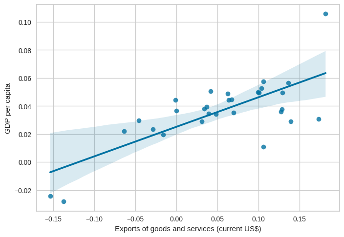
By examining the scatter plot, we can observe the relationship between exports and GDP per capita. A positive correlation or upward trend suggests that higher exports are associated with higher GDP per capita, indicating the importance of international trade for economic prosperity

Unemployment rate

Another vital factor that significantly influences a country’s economic well-being is the unemployment rate. The unemployment rate is a crucial indicator that measures the percentage of the labor force without employment but actively seeking work. It plays a pivotal role in understanding the overall health of an economy and its impact on GDP per capita. Let’s explore how the unemployment rate affects GDP per capita and how we can visualize this relationship

sns.regplot(
            data=reg_pct, 
            x='Unemployment rate', 
            y='GDP per capita'
            )

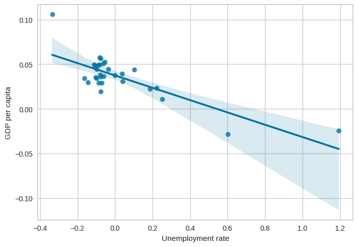
Analyzing the scatter plot helps us visualize the relationship between the unemployment rate and GDP per capita. A negative correlation or a downward trend suggests that lower unemployment rates are associated with higher GDP per capita, indicating the positive impact of a vibrant labor market on economic prosperity.

data_select = data[['GDP per capita',"Unemployment rate"]].pct_change()
plot_hist(data_select) 

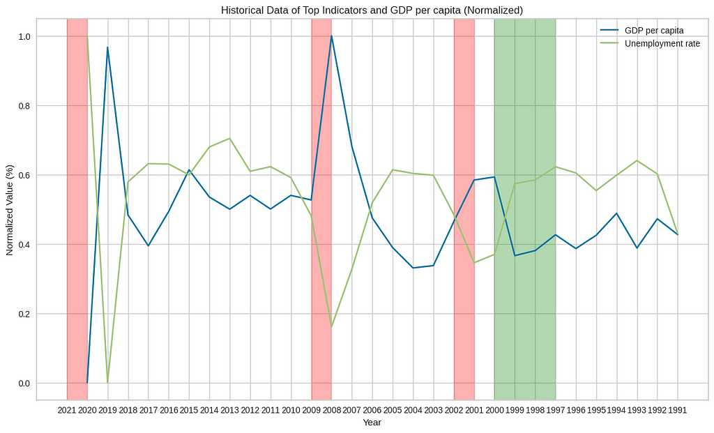
Exploring Historical Events

Understanding the relationships between historical events can provide valuable insights into how these events influenced indicators such as the unemployment rate and gross fixed capital formation, ultimately affecting GDP per capita. Understanding these dynamics helps us build a better model

data_select = data[['GDP per capita',
                    'Exports of goods and services (current US$)', 
                    'Gross fixed capital formation (current US$)']]
plot_hist(data_select)   

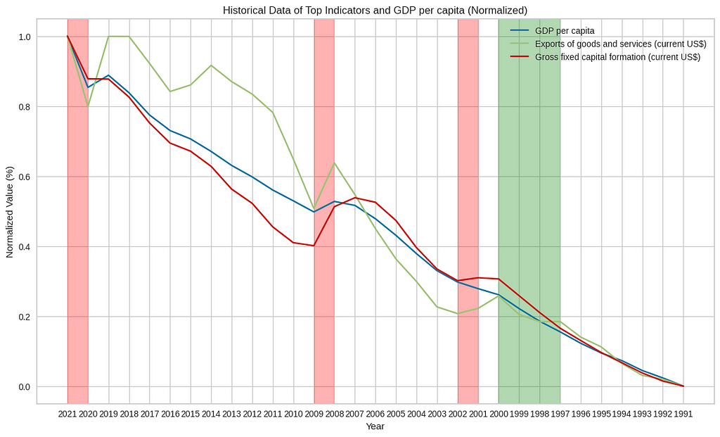
By examining the graph, we can expect the following observations during these events:

• Dot-com boom (1997–2000): We may notice a sharp increase in GDP per capita and gross fixed capital formation during this period. The unemployment rate may have been relatively low, reflecting the high demand for skilled workers in the technology and internet sectors.
• Dot-com bust (2001–2002): The graph may show a decline in GDP per capita and gross fixed capital formation as the dot-com bubble burst. This period might have experienced a notable increase in the unemployment rate as many technology companies struggled or went bankrupt.
• The financial crisis (2008–2009): The graph is likely to exhibit a significant drop in GDP per capita, gross fixed capital formation, and a sharp rise in the unemployment rate. The financial crisis led to a global recession, with many businesses failing and financial markets experiencing severe turmoil.
• Covid-19 pandemic (2020–2021): The graph might display a sharp decline in GDP per capita, gross fixed capital formation, and a substantial increase in the unemployment rate. The Covid-19 pandemic caused widespread disruptions to economies worldwide, with lockdown measures and reduced economic activity impacting various sectors.

FDI

Foreign Direct Investment (FDI) plays a crucial role in shaping a country’s GDP. When GDP and FDI align and reach their peaks, it signifies a period of robust economic growth and attractiveness for foreign investment.

data_delta = data[['GDP per capita','Foreign direct investment, net inflows (BoP, current US$)']].pct_change().dropna()
scaler = MinMaxScaler()
data_delta = pd.DataFrame(scaler.fit_transform(data_delta), columns=data_delta.columns, index=data_delta.index)

fdi = data_delta['Foreign direct investment, net inflows (BoP, current US$)']

plt.figure(figsize=(14, 8))
plt.plot(data_delta.index, fdi, label='Foreign direct investment, net inflows (BoP, current US$)')
plt.plot(data_delta.index, data_delta['GDP per capita'], label='GDP per capita', linewidth=2, linestyle='--')

fdi_peak_indices = argrelextrema(np.array(fdi), np.greater)
gdp_peak_indices = argrelextrema(np.array(data_delta['GDP per capita']), np.greater)

matching_indices = set(fdi_peak_indices[0]).intersection(gdp_peak_indices[0])
for peak_index in matching_indices:
    if fdi.iloc[peak_index] > 0.6 and data_delta['GDP per capita'].iloc[peak_index] > 0.5:
        x = fdi.index[peak_index]
        y1 = fdi.iloc[peak_index]
        y2 = data_delta['GDP per capita'].iloc[peak_index]
        plt.axvspan(str(int(x)-1),str(int(x)+1), alpha=0.3, color='red')

plt.xlabel('Year')
plt.ylabel('Normalized Value (%)')
plt.title('Historical Data of FDI and GDP per capita (Normalized)')
plt.legend()
plt.show()

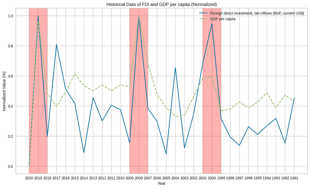
When the graph of GDP and Foreign Direct Investment (FDI) align and reach their peaks, it indicates a positive relationship and several key insights. It suggests strong economic growth, driven by high levels of FDI flowing into the country. This alignment signifies an attractive investment environment, with foreign investors having confidence in the country’s economic prospects.

Modeling

To model the data effectively, we utilize the PyCaret library, which simplifies machine learning tasks. We set up a regression model, compare various algorithms, and tune the best-performing model using cross-validation. By leveraging the power of ensemble modeling, we combine the predictions of multiple models to create an ensemble model, resulting in improved accuracy and robustness.

Here’s an example section of code that demonstrates how to set up a regression model using PyCaret:

model_setup = setup(reg_pct, 
                    target = "GDP per capita", 
                    session_id = 123,
                    use_gpu=True)

Output:
+-------+-----------------------------+------------------+
| index |         Description         |      Value       |
+-------+-----------------------------+------------------+
|     0 | Session id                  | 123              |
|     1 | Target                      | GDP per capita   |
|     2 | Target type                 | Regression       |
|     3 | Original data shape         | (30, 7)          |
|     4 | Transformed data shape      | (30, 7)          |
|     5 | Transformed train set shape | (21, 7)          |
|     6 | Transformed test set shape  | (9, 7)           |
|     7 | Numeric features            | 6                |
|     8 | Preprocess                  | True             |
|     9 | Imputation type             | simple           |
|    10 | Numeric imputation          | mean             |
|    11 | Categorical imputation      | mode             |
|    12 | Fold Generator              | KFold            |
|    13 | Fold Number                 | 10               |
|    14 | CPU Jobs                    | -1               |
|    15 | Use GPU                     | True             |
|    16 | Log Experiment              | False            |
|    17 | Experiment Name             | reg-default-name |
|    18 | USI                         | 3afd             |
+-------+-----------------------------+------------------+

By executing this code, PyCaret will automatically perform essential data preprocessing steps, such as handling missing values, feature scaling, and feature transformation. It will also create a validation set and initialize the environment for subsequent modeling steps.

After setting up the regression model using PyCaret, the next step is to compare different regression models to identify the best-performing one for our dataset. PyCaret provides a convenient function called compare_models() that automates the process of training and evaluating multiple regression models. Here’s an example section of code that demonstrates how to compare models

base_model = compare_models(fold=2)

Output:
+----------+---------------------------------+--------+--------+--------+----------+--------+--------+----------+
|  Model   |              Model              |  MAE   |  MSE   |  RMSE  |    R2    | RMSLE  |  MAPE  | TT (Sec) |
+----------+---------------------------------+--------+--------+--------+----------+--------+--------+----------+
| br       | Bayesian Ridge                  | 0.0109 | 0.0002 | 0.0141 |   0.4613 | 0.0108 | 0.3651 |   0.0800 |
| xgboost  | Extreme Gradient Boosting       | 0.0111 | 0.0002 | 0.0148 |   0.3462 | 0.0102 | 0.3746 |   1.0650 |
| dt       | Decision Tree Regressor         | 0.0124 | 0.0003 | 0.0153 |   0.3129 | 0.0116 | 0.4061 |   0.2300 |
| ridge    | Ridge Regression                | 0.0119 | 0.0003 | 0.0164 |   0.2993 | 0.0103 | 0.4137 |   0.1250 |
| rf       | Random Forest Regressor         | 0.0122 | 0.0003 | 0.0166 |   0.2049 | 0.0100 | 0.4453 |   0.5650 |
| omp      | Orthogonal Matching Pursuit     | 0.0132 | 0.0004 | 0.0177 |   0.1644 | 0.0112 | 0.4422 |   0.0800 |
| et       | Extra Trees Regressor           | 0.0125 | 0.0003 | 0.0165 |   0.1604 | 0.0103 | 0.4434 |   0.5800 |
| ada      | AdaBoost Regressor              | 0.0124 | 0.0003 | 0.0163 |   0.1199 | 0.0110 | 0.4339 |   0.3050 |
| gbr      | Gradient Boosting Regressor     | 0.0136 | 0.0003 | 0.0171 |   0.0875 | 0.0117 | 0.4839 |   0.2650 |
| knn      | K Neighbors Regressor           | 0.0140 | 0.0004 | 0.0193 |  -0.1144 | 0.0122 | 0.5176 |   0.1800 |
| lasso    | Lasso Regression                | 0.0153 | 0.0005 | 0.0202 |  -0.1303 | 0.0115 | 0.5137 |   0.0900 |
| en       | Elastic Net                     | 0.0153 | 0.0005 | 0.0202 |  -0.1303 | 0.0115 | 0.5137 |   0.0800 |
| llar     | Lasso Least Angle Regression    | 0.0153 | 0.0005 | 0.0202 |  -0.1303 | 0.0115 | 0.5137 |   0.0800 |
| lightgbm | Light Gradient Boosting Machine | 0.0153 | 0.0005 | 0.0202 |  -0.1303 | 0.0115 | 0.5137 |   0.1300 |
| dummy    | Dummy Regressor                 | 0.0153 | 0.0005 | 0.0202 |  -0.1303 | 0.0115 | 0.5137 |   0.2150 |
| huber    | Huber Regressor                 | 0.0241 | 0.0029 | 0.0438 |  -3.2428 | 0.0329 | 0.8584 |   0.0850 |
| lr       | Linear Regression               | 0.0249 | 0.0032 | 0.0452 |  -3.5208 | 0.0340 | 0.8919 |   0.0800 |
| par      | Passive Aggressive Regressor    | 0.0346 | 0.0013 | 0.0362 |  -4.9714 | 0.0355 | 1.0000 |   0.0850 |
| lar      | Least Angle Regression          | 0.0666 | 0.0208 | 0.1197 | -31.1585 | 0.0847 | 2.4717 |   0.0800 |
+----------+---------------------------------+--------+--------+--------+----------+--------+--------+----------+

By setting fold=2, PyCaret will perform a 2-fold cross-validation, splitting the data into two subsets and using each subset as a validation set in turn while training the model on the remaining data. This approach allows for a reasonable evaluation of the model’s performance while still utilizing as much data as possible for training.

After comparing and selecting a base regression model using compare_models(), the next step is to further enhance its performance through hyperparameter tuning. PyCaret provides a convenient function called tune_model() that automates the process of optimizing the hyperparameters of a model using cross-validation. Here’s an example section of code that demonstrates how to tune the hyperparameters of the base model using PyCaret:

tuned_model = tune_model(base_model,fold=2) 

+-------+--------+--------+--------+--------+--------+--------+
| Fold  |  MAE   |  MSE   |  RMSE  |   R2   | RMSLE  |  MAPE  |
+-------+--------+--------+--------+--------+--------+--------+
| 0     | 0.0069 | 0.0001 | 0.0080 | 0.4288 | 0.0078 | 0.2981 |
| 1     | 0.0121 | 0.0002 | 0.0157 | 0.6909 | 0.0138 | 0.3355 |
| Mean  | 0.0095 | 0.0002 | 0.0118 | 0.5598 | 0.0108 | 0.3168 |
| Std   | 0.0026 | 0.0001 | 0.0038 | 0.1311 | 0.0030 | 0.0187 |
+-------+--------+--------+--------+--------+--------+--------+

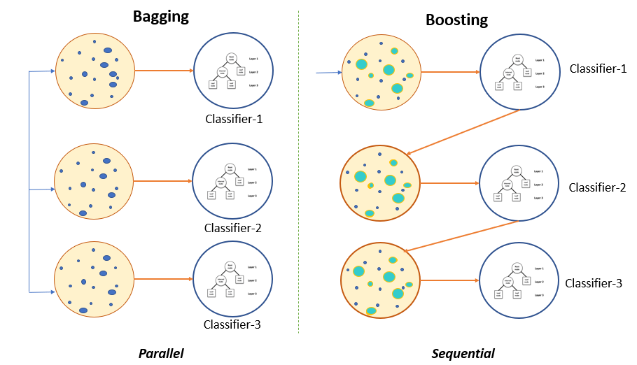
After tuning the regression model, another effective technique to improve its performance is to create an ensemble model. Ensemble models combine the predictions of multiple individual models to make more accurate and robust predictions. PyCaret provides a convenient function called ensemble_model() to build an ensemble model from a tuned base model. Here’s an example section of code that demonstrates how to create an ensemble model:

ensembled_model = ensemble_model(tuned_model,fold=2,method="Boosting")

+-------+--------+--------+--------+--------+--------+--------+
| Fold  |  MAE   |  MSE   |  RMSE  |   R2   | RMSLE  |  MAPE  |
+-------+--------+--------+--------+--------+--------+--------+
| 0     | 0.0077 | 0.0001 | 0.0096 | 0.1744 | 0.0093 | 0.3669 |
| 1     | 0.0129 | 0.0002 | 0.0158 | 0.6871 | 0.0152 | 0.3640 |
| Mean  | 0.0103 | 0.0002 | 0.0127 | 0.4307 | 0.0123 | 0.3655 |
| Std   | 0.0026 | 0.0001 | 0.0031 | 0.2563 | 0.0029 | 0.0015 |
+-------+--------+--------+--------+--------+--------+--------+

Creating an ensemble model using PyCaret’s ensemble_model() function allows for the aggregation of predictions from multiple models, resulting in a more robust and accurate overall prediction. The ensemble model captures complex patterns and relationships in the data more effectively, leading to improved decision-making and potentially better outcomes.

Assessing Model Performance

Once you have tuned your regression model using PyCaret, it’s crucial to evaluate its performance visually. PyCaret provides a powerful function called plot_model() that allows you to generate various visualizations to assess the model’s performance.

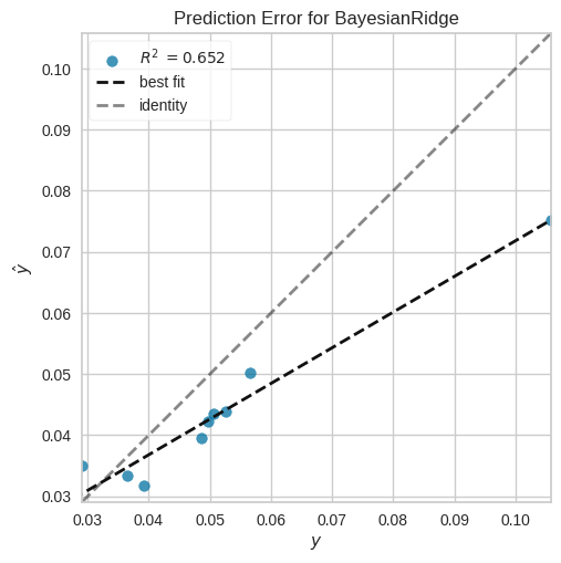
plot_model(tuned_model, plot = 'error')

plot_model(ensembled_model, plot = 'error')

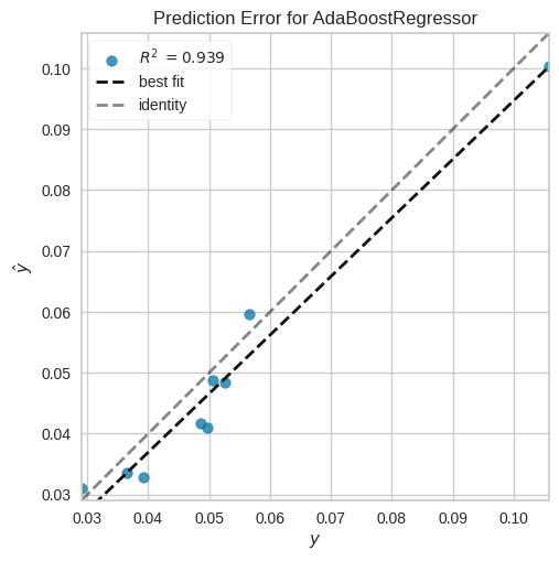
When comparing the performance of the ensemble model to individual models, there is typically a substantial improvement in the error rate. The ensemble model demonstrates a significant reduction in error rate compared to individual models. This improvement signifies its ability to provide more accurate predictions.

The ensemble model’s predictions exhibit reduced deviations from the best-fit line, implying that it captures the underlying patterns and relationships in the data more accurately. This improvement can be attributed to the ensemble model’s ability to combine the strengths of multiple individual models and mitigate their weaknesses, resulting in enhanced predictive accuracy.

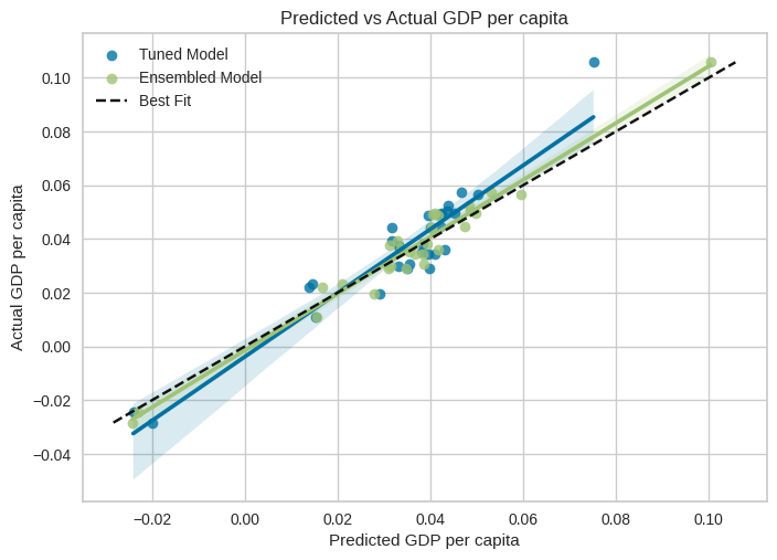
Visualizing Predicted vs Actual GDP per capita

To gain insights into the performance of the tuned model and the ensemble model, we can visualize the predicted values against the actual values of GDP per capita. The following code snippet demonstrates how to plot the predicted vs actual GDP per capita

tuned_predictions = predict_model(tuned_model, data=reg_pct)
ensembled_predictions = predict_model(ensembled_model, data=reg_pct)

sns.regplot(x=tuned_predictions["prediction_label"], y=reg_pct["GDP per capita"], label="Tuned Model")
sns.regplot(x=ensembled_predictions["prediction_label"], y=reg_pct["GDP per capita"], label="Ensembled Model")

best_fit_x = np.linspace(reg_pct["GDP per capita"].min(), reg_pct["GDP per capita"].max(), 100)
best_fit_y = best_fit_x

plt.plot(best_fit_x, best_fit_y, 'k--', label="Best Fit")

plt.xlabel("Predicted GDP per capita")
plt.ylabel("Actual GDP per capita")
plt.title("Predicted vs Actual GDP per capita")

plt.legend()
plt.show()

combined_data = pd.concat([tuned_predictions["prediction_label"], ensembled_predictions["prediction_label"], reg_pct["GDP per capita"]], axis=1)
combined_data.columns = ["Tuned Model Predictions", "Ensembled Model Predictions", "GDP per capita"]
combined_data.index = data[1:].reindex(index=data[:-1].index[::-1]).index
combined_data = combined_data.reset_index()

plt.plot(combined_data["date"],combined_data["GDP per capita"], label="Ground Truth")
plt.plot(combined_data["date"],combined_data["Tuned Model Predictions"],  label="Tuned Model")
plt.plot(combined_data["date"],combined_data["Ensembled Model Predictions"], label="Ensembled Model")

plt.xlabel("Years")
xticks_locs = plt.xticks()[0] 
new_xticks_locs = xticks_locs[::2] 
new_xticks_labels = [combined_data['date'][int(i)] if i < len(combined_data['date']) else '' for i in new_xticks_locs] 
plt.xticks(new_xticks_locs, new_xticks_labels) 

plt.legend()
plt.show()

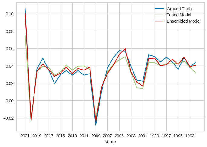
As observed from the plotted predicted vs actual GDP per capita values, it is evident that the ensemble model has improved the modeling performance compared to the tuned model alone. The ensemble model’s predicted values align more closely with the actual GDP per capita values, indicating a better fit

Colab

Colab Link

Conclusion

In conclusion, this tutorial showcased the value of using voting models, particularly ensemble models, in handling small economic datasets in econometrics. By leveraging machine learning techniques, we unlocked insights from economic data and demonstrated the importance of factors like exports, investment, and the unemployment rate in influencing GDP per capita. Through visualization and modeling, we provided a comprehensive guide to harnessing voting models and improving predictive accuracy in econometric analysis. These techniques empower economists and policymakers to make informed decisions and gain deeper insights into economic dynamics

Unlocking the Potential of Machine Learning in Econometrics: Ensemble Models for Improved… was originally published in Google Developer Experts on Medium, where people are continuing the conversation by highlighting and responding to this story.