A beginner-friendly deep dive into how Mixture-of-Experts works, why it matters, and how to build one in pure JAX/Flax.
TL;DR
We built nano-moe-jax — a lightweight, educational Mixture-of-Experts (MoE) transformer that trains a character-level language model on a single GPU (or even CPU).
Install it with:
pip install nano-moe-jax
Train on Shakespeare in one command. Learn MoE from first principles.
Why This Post Exists
Mixture-of-Experts (MoE) powers some of the largest models in the world — yet most explanations are either:
- Extremely theoretical
- Or buried inside trillion-parameter research papers
So instead of scaling to trillions… we scaled down.
This article walks you through building a 2.4M parameter nano-MoE transformer completely from scratch in JAX — while explaining:
- What MoE actually is
- Why it works
- How routing works
- Why load balancing is critical
- And how to train one yourself
1. What is Mixture of Experts?
Imagine a team of specialists.
Instead of asking every specialist to look at every problem, you hire a manager. The manager looks at each problem and says:
“Expert #2 and Expert #4 — this one’s yours.”
That’s Mixture-of-Experts.
Core Components
- Experts → Independent feed-forward networks
- Router (Gate) → Learns which experts to activate
- Sparse activation → Only a subset of experts run per token
In a standard transformer:
Every token uses every parameter.
In MoE:
The model has more total parameters — but activates only a fraction per token.
That’s the magic.
More capacity.
Similar compute.
2. Why MoE Matters
MoE architectures power some of the most advanced models today:
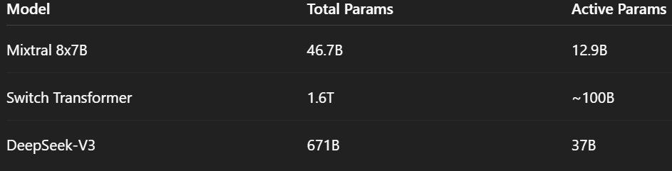
Notice something?
Total parameters are often 3–16× larger than active parameters.
This means:
- You get massive capacity
- Without proportional increase in FLOPs
- And with specialization emerging naturally
3. Architecture Overview
Our NanoMoE is a GPT-style autoregressive transformer.
The only difference?
We replace the standard Feed-Forward Network (FFN) inside each transformer block with an MoE layer.
Default Hyperparameters

Total parameters: 2,409,025
Small enough to train on CPU.
Large enough to demonstrate real MoE behavior.

4. The Building Blocks
4.1 Expert Feed-Forward Network
Each expert is a simple 2-layer MLP:
class ExpertFFN(nn.Module):
    d_ff: int
    d_model: int

    @nn.compact
    def __call__(self, x):
        x = nn.Dense(self.d_ff)(x)
        x = nn.gelu(x)
        x = nn.Dense(self.d_model)(x)
        return x
Why GELU?
Because modern transformers (GPT-2, BERT, LLaMA, etc.) use it.
It provides smoother gradients than ReLU.
4.2 Multi-Head Causal Self-Attention
This part is standard transformer attention.
Causal masking ensures:
Token at position t can only attend to tokens ≤ t.
That’s what makes it autoregressive.
5. The Router — The Brain of MoE
The router decides:
“Which experts should process this token?”
Top-K Routing Process
- Project token → n_experts logits
- Select top-K experts
- Softmax only over selected experts
- Run selected experts
- Weighted sum of outputs
Example:
logits = nn.Dense(n_experts)(token)
top_values, top_indices = jax.lax.top_k(logits, k=2)
gates = jax.nn.softmax(top_values)
output = gates[0] * expert_3(token) + gates[1] * expert_1(token)
Important detail:
We normalize only over selected experts — not all experts.
This keeps routing sparse and efficient.
6. Load Balancing — Preventing Expert Collapse
The biggest MoE failure mode?
Expert collapse.
Without constraints, the router might send almost all tokens to 1 expert.
Result:
- One overloaded expert
- Others unused
- Training instability
To fix this, we add an auxiliary loss inspired by the Switch Transformer:
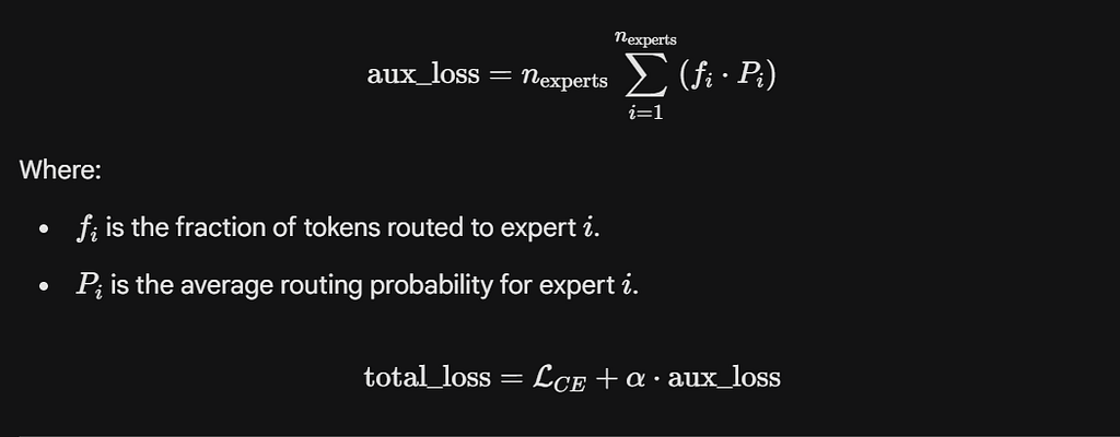
We use:
α = 0.01
Small enough not to dominate training.
Strong enough to keep experts balanced.
7. Full Model Flow
Each transformer block:
x → LayerNorm
  → Self-Attention
  → Residual Add
  → LayerNorm
  → MoE Layer
  → Residual Add
We use pre-norm instead of post-norm:
output = x + SubLayer(LayerNorm(x))
Why pre-norm?
- Better gradient flow
- More stable training
- Standard in modern LLMs
8. Training Pipeline (JAX Magic)
Our entire training step is wrapped in @jax.jit.
What happens?
- First step → XLA compilation
- All subsequent steps → optimized kernel execution
- jax.grad handles automatic differentiation
@jax.jit
def train_step(state, x, y):
    def loss_fn(params):
        logits, aux_loss = model.apply({"params": params}, x)
        ce_loss = cross_entropy(logits, y)
        return ce_loss + 0.01 * aux_loss
    grads = jax.grad(loss_fn)(state.params)
    state = state.apply_gradients(grads=grads)
    return state
That’s it.
Clean. Functional. Efficient.
9. Results — Training on Shakespeare
Dataset: Tiny Shakespeare (~1.1M characters)
Steps: 5,000
Final metrics:

Observations
- Loss dropped from 4.23 → 1.54
- Aux loss stayed stable (~4.0 = balanced routing)
- Small train-val gap → minimal overfitting
- 2.4M parameters trained in ~4h on CPU
For a nano-MoE model — that’s solid.
10. Code Structure
nano_moe/
├── config.py
├── layers.py
├── model.py
├── train.py
├── utils.py
The MoE layer works like this:
def __call__(self, x):
    gates, indices, aux_loss = Router(...)(x)
    expert_outputs = [expert(x) for expert in experts]
    expert_outputs = jnp.stack(expert_outputs)
    selected = expert_outputs[indices]
    output = sum(gates * selected)
    return output, aux_loss
Because this is nano-scale, we simply run all experts and select afterward.
At large scale, experts are sharded across devices.
11. Dense vs MoE
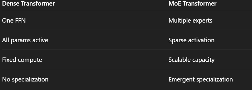
MoE lets you increase model capacity without increasing compute per token.
That’s why trillion-parameter models are feasible.
12. Try It Yourself
Install
pip install nano-moe-jax
Or Clone
git clone https://github.com/carrycooldude/MoE-JAX.git
cd MoE-JAX
pip install -e .
python examples/train_shakespeare.py
Use as Library
config = NanoMoEConfig(
    vocab_size=65,
    n_layers=6,
    n_experts=8,
    top_k=2,
    d_model=256,
)
model = NanoMoE(config=config)
What You Learned
- MoE = Experts + Router + Sparse activation
- Load balancing prevents expert collapse
- Pre-norm improves stability
- JAX makes routing + differentiation elegant
- Even a 2.4M parameter MoE demonstrates real scaling behavior
What to Explore Next
- Increase number of experts (8, 16, 32)
- Try expert parallelism
- Experiment with routing strategies
- Train on larger datasets
- Implement token dropping
Resources
- Repo: https://github.com/carrycooldude/MoE-JAX
- PyPI: https://pypi.org/project/nano-moe-jax/
- Switch Transformer Paper
- Mixtral Paper
- JAX & Flax Documentation
If this helped you understand MoE better, consider starring the repo.
Built with JAX, Flax, and Optax.
![]()
Building a Nano Mixture-of-Experts (MoE) Language Model in JAX from Scratch was originally published in Google Developer Experts on Medium, where people are continuing the conversation by highlighting and responding to this story.