Linear regression is a simple yet powerful method in machine learning used to model the relationship between a dependent variable (target) and one or more independent variables (predictors). In this article, we will implement a simple linear regression using NumPy, a powerful library for scientific computing in Python. We will cover the different equations necessary for this implementation: the model, the cost function, the gradient, and gradient descent.
1. Linear Regression Model
The linear regression model can be represented by the following equation:

y=Xθ
where:
- X is the matrix of predictors.
- θ is the vector of parameters (coefficients).
2. Cost Function
The cost function in linear regression is often the sum of squared errors (mean squared error). It measures the difference between the values predicted by the model and the actual values.

3. Gradient
The gradient of the cost function with respect to the parameters
θ is necessary to minimize the cost function using gradient descent. The gradient is calculated as follows:
![]()
4. Gradient Descent
Gradient descent is an iterative optimization method used to minimize the cost function. The parameter update equation is:
![]()
5. Implementation with NumPy
importing libraries
import numpy as np
import pandas as pd
import matplotlib.pyplot as plt
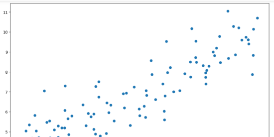
Generate example data
np.random.seed(42)
m = 100
x = 2 * np.random.rand(m, 1)
y = 4 + 3 * x + np.random.randn(m, 1)
plt.figure(figsize=(12, 8))
plt.scatter(x, y)

Add a bias term (column of 1s) to X
X = np.hstack((x, np.ones(x.shape)))
X.shape
(100, 2)
Initialize the parameters θ to random values
theta = np.random.randn(2, 1)
Model function
def model(X, theta):
    return X.dot(theta)

plt.scatter(x[:, 0], y)
plt.scatter(x[:, 0], model(X, theta), c='r')

Cost function
def cost_function(X, y, theta):
    m = len(y)
    return 1/(2*m) * np.sum((model(X, theta) - y)**2)

cost_function(X, y, theta)
16.069293038191518
Gradient et Gradient descent
def grad(X, y, theta):
    m = len(y)
    return 1/m * X.T.dot(model(X, theta) - y)

def gradient_descent(X, y, theta, learning_rate, n_iter):
    cost_history = np.zeros(n_iter)
    for i in range(0, n_iter):
        theta = theta - learning_rate * grad(X, y, theta)
        cost_history[i] = cost_function(X, y, theta)

    return theta, cost_history
n_iterations = 1000
learning_rate = 0.01

final_theta, cost_history = gradient_descent(X, y, theta, learning_rate, n_iterations)

final_theta
array([[2.79981142],
[4.18146098]])
predict = model(X, funal_theta)

plt.scatter(x[:, 0], y)
plt.scatter(x[:, 0], predict, c='r')

Learning curve
plt.plot(range(n_iterations), cost_history)

This implementation demonstrates how the fundamental concepts of linear regression, such as the model, cost function, gradient, and gradient descent, can be implemented using NumPy. This basic understanding is essential for advancing to more complex machine learning models.
Feel free to explore further by adjusting hyperparameters, adding more features, or trying other optimization techniques to improve your linear regression model.